System Matrix and Phantom Dataset Acquired by FFL Rotational Imaging

1. Dataset Overview

This dataset contains system matrix and phantom data acquired using a self-developed device (PR-MPI system). The device is a Field-Free Line (FFL)-based system. Detailed information about the device can be found in the article A compact low-power magnetic particle imaging scanner based on a permanent-magnet field-free-line generator with high gradient, https://doi.org/10.1063/5.0324735.

Data acquisition was performed using the FFL rotational imaging method described in the above article (Fig. 6). The FFL was excited and scanned along the y direction, and two-dimensional scanning in the y-z plane was achieved by rotating the FFL. Considering the complexity of rotating the permanent magnets, the relative rotation of the FFL was achieved by rotating the phantom. The basic scanning parameters are listed in the table below.

1) System Matrix Data

A total of two complete FFL rotational system matrices were acquired, differing in the tracer used. Synomag-70 and Perimag particles were used for acquisition, and the corresponding data are stored in the syno and peri folders, respectively. Each folder contains the raw particle time-domain signal data and corresponding background time-domain signal data acquired at 20 FFL angles. The FFL angles were calculated using the golden-angle method:

°                                              (1)

where  represents the -th angle, °, and mod(∙) denotes the modulo operation. The relative rotation of the FFL was achieved by rotating the phantom; therefore, the coordinates at the current angle  were updated according to the calculated angle (see Fig. 7). Based on the updated coordinates, the 19×19 positions in the FOV were traversed using point-by-point scanning, with the scanning order from right to left and from top to bottom, as shown in the figure below.

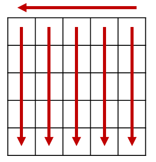
The data organization of the two folders is similar. Taking the syno folder as an example, it contains two subfolders, Particle and Background, corresponding to the particle time-domain signals and background time-domain signals, respectively. The Particle folder contains 20 “.mat” files named open_sm_syno_angle_{i}_sig.mat,  representing the -th angle  obtained from Eq. (1). Each mat file contains a 2,500,000×361 matrix, where 361=19×19 represents the number of discrete positions within the FOV. Therefore, each 2,500,000×1 data vector corresponds to the raw time-domain signal at one discrete spatial position in the FOV. The Background folder also contains 20 “.mat” files named open_sm_syno_angle_{i}_back.mat. Their stored contents are similar to those in the Particle folder.

The Particle folder stores the particle signals of the delta phantom at different discrete positions in the FOV (with the background subtracted), while the Background folder stores the corresponding background signals (without particle signals). The two signals correspond one-to-one along the 361 dimension.

2) Phantom Data

To be uploaded and updated

2. Data Usage

1) Basic Reconstruction Procedure

• Fourier Transform. The raw signals are in the time domain. First, the system matrix and phantom signals can be separately transformed into the frequency domain to obtain the corresponding frequency-domain signals.
• Frequency Selection. Since particle information is mainly contained in the harmonics, frequency selection can be performed on the frequency-domain signals of the system matrix and phantom (e.g., selecting the 2^nd-10^th harmonics for reconstruction). Alternatively, based on the provided system matrix background signals, frequency points with an SNR greater than a certain threshold can be calculated and selected accordingly.
• Image Reconstruction. The signals from the 20 FFL angles are concatenated to obtain the complete system matrix, and the same operation is performed on the phantom signals to obtain the reconstructed image.

3. Potential Applications of the Dataset

This dataset can be used for:

1) Validation of MPI Image Reconstruction Algorithms. The performance of different reconstruction algorithms can be evaluated, including Kaczmarz, Tikhonov regularization, deep learning-based reconstruction, etc.

2) System Matrix Processing Research. This includes frequency-domain analysis, frequency-point selection, system matrix compression, system matrix quality improvement and super resolution, etc.

3) Signal Enhancement and Denoising Experiments. This includes denoising of raw MPI time-domain signals, signal enhancement, deep learning-based signal recovery, etc.

Citation:

Zechen Wei et al., A compact low-power magnetic particle imaging scanner based on a permanent-magnet field-free-line generator with high gradient, Review of Scientific Instruments, 2026, 97 (6), https://doi.org/10.1063/5.0324735.